Strategies for Greedy Vertex Colouring

In the previous post we showed that a greedy vertex colouring of a graph \(G\) uses at most \(\Delta(G) + 1\) colours. This sounds good until we realise that graphs can have chromatic number much lower than the maximum degree.

The crown graphs, sometimes called Johnson graphs are complete bipartite graph \(K_{2n, 2n}\) with a one-factor removed.

import networkx as nx

def one_factor(n):
    """The one-factor we remove from K_{2n,2n} to make a crown graph."""
    return zip(range(n),range(2*n - 1, n - 1, -1))

def crown_graph(n):
    """K_{n, n} minus one-factor."""
    G = nx.complete_bipartite_graph(n, n)
    G.remove_edges_from(one_factor(n))
    return G

G = crown_graph(6)

setfigsize(6,6)

options = {
  'with_labels': False,
  'node_size': 250,
  'width': 0.5,
}

nx.draw_circular(G, node_color = 'black', **options)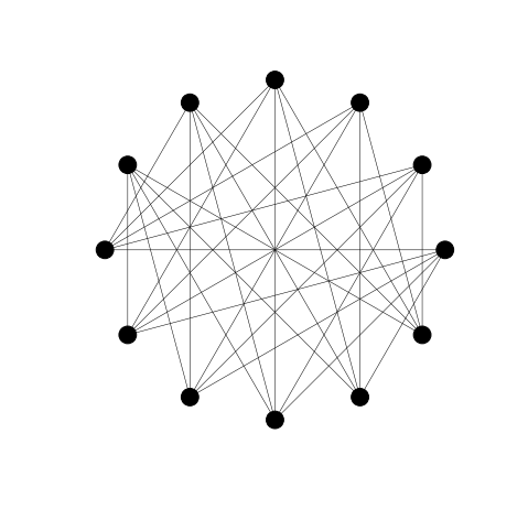

png

Crown graphs are bipartite and hence 2-colourable.

vcolour(G)
nx.draw_circular(G, node_color = colours(G), **options)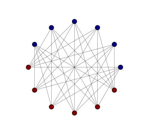

png

However, the maximum degree of a crown graph \(G\) of order \(2n\) is \(n - 1\) and, with some vertex orderings, a greedy colouring of \(G\) uses \(\Delta(G) + 1 = n\) colours.

import itertools

def bad_order(n):
    """Visit nodes in the order of the missing one-factor."""
    return itertools.chain.from_iterable(one_factor(n))

clear_colouring(G)
vcolour(G, nodes = bad_order(6))
nx.draw_circular(G, node_color = colours(G), **options)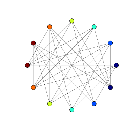

png

We might ask, what vertex orderings lead to colourings with fewer colours? The following theorem of Dominic A. Welsh and Martin B. Powell is pertinent.

Theorem (Welsh, Powell)

Let \(G\) be a graph of order \(n\) whose vertices are listed in the order \(v_{1}, v_{2}, ... v_{n}\) so that \(\operatorname{deg} v_{1} \geq \operatorname{deg} v_{2}\geq \dots \geq\operatorname{deg} v_{n}\). Then \(\chi(G) \leq 1 + \min_{1 \leq i \leq n}\{\max{\{i - 1, \operatorname{deg} v_{i}\}\}} = \min_{1\leq i\leq n}\{\max{\{i, 1 + \operatorname{deg} v_{i}}\}\}\)

In the case of regular graphs, like the crown graphs, this theorem reduces to the \(\Delta(G) + 1\) upper-bound on the chromatic number. For graphs that are not regular this result suggests that we can get a tighter bound on the chromatic number by considering orderings of vertices in non-increasing degree order.

The Grotzsch graph is an irregular graph that plays an important role in the study of graph colouring. Unfortunately, it is not one of the named graphs in NetworkX. We can, however, download it from the House of Graphs as a file in graph6 format. Then we can use the read_graph6 function to read it into a NetworkX graph.

G = nx.read_graph6('graph_1132.g6')

nx.draw_circular(G, node_color = 'black', **options)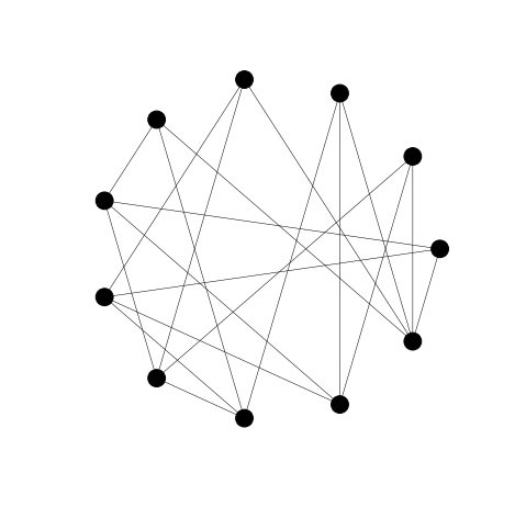

png

We can compute the bound from the Welsh-Powell theorem.

def welsh_powell_number(G, nodes = None):
    """Calculate bound from Welsh-Powell theorem with nodes in given order."""
    if nodes == None: nodes = G.nodes()
    if len(nodes) == 0: return 0
    else:
        return 1 + min([max(i, G.degree(nodes[i])) for i in range(len(nodes))])

welsh_powell_number(G)
4

which is a significant improvement over the \(\Delta(G) + 1 = 6\) bound. In fact, the chromatic number of the Grotzsch graph is 4 and a greedy colouring with 4 colours can be found.

vcolour(G)
nx.draw_circular(G, node_color = colours(G), **options)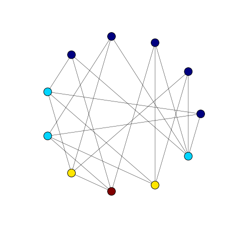

png

We might suspect then that a good vertex colouring strategy is greedy colouring with vertices in non-increasing degree order. In the next section we devise a small test of this claim.

Greedy Strategies for Colouring Small Graphs

NetworkX comes with a collection of all unlabelled, undirected graphs on seven or fewer vertices based on Read and Wilson (2005) . The experiment below colours every graph in this collection using four different vertex orderings: in order, random order, decreasing degree order and increasing degree. In order is the order ordering of vertices in the data representation of the graph. In the case of NetworkX this just means that we colour vertices in the order they appear in G.nodes(). Random order just means that we first shuffle this list using random.shuffle. The other orderings are defined by the degree_order function below.

def degree_order(G, reverse = False):
    """Vertices of G, ordered by degree."""
    return sorted(G.nodes(), key = G.degree, reverse = reverse)

In the following code extract we iterate over the graphs in graphs_atlas_g() colouring each graph with each of the four above mentioned vertex ordering strategies. We calculate the number of colours used by each colouring and, at the end, we print out the totals of these numbers over all graphs.

import networkx as nx
import random

graphs = nx.graph_atlas_g()

colours_used = {'inorder': 0, 'random': 0, 'decdeg': 0, 'incdeg': 0}

for G in graphs:

    nodes = G.nodes()
    inorder_nodes = nodes
    random_nodes = random.shuffle(nodes)
    
    orderings = {'inorder': nodes,
                 'random': random_nodes,
                 'decdeg': degree_order(G, reverse = True),
                 'incdeg': degree_order(G)}
    
    for ordering in orderings:
        vcolour(G, nodes = orderings[ordering])
        colours_used[ordering] += ncolours(G)
        clear_colouring(G)

Ordering	Colours used
in order	4255
random order	4252
descending degree order	4120
ascending degree order	4468

We can see that the best ordering to use in this case is the ordering claimed in Welsh and Powell’s theorem. Ordering vertices by their degree from highest to lowest. The worst case is the reverse ordering and randomised and natural orderings lie somewhere in between.

References

Read, Ronald C., and Robin J. Wilson. 2005. An Atlas of Graphs (Mathematics). USA: Oxford University Press, Inc.